
In this post I share a small example about how to find the most frequent words in Tripadvisor reviews. I followed some examples that I mentioned in the references and I build this resume for those who are starting in this topics.
#Building a corpus
library(tm)
library(NLP)
data<- VectorSource(data) #converted our vector to a Source object
data <- VCorpus(data) #to create our volatile corpus.

#Cleaning and preprocessing of the text
#After obtaining the corpus, usually, the next step will be cleaning and preprocessing of the text.
library(tm)
library(qdap) # qdap package offers other text cleaning functions
data<-tolower(data) #all lowercase
data<-removePunctuation(data) #remove punctuation
data<-removeNumbers(data) #remove numbers
data<-stripWhitespace(data) # Remove whitespace
#cleaning
data<-bracketX(data) # Remove text within brackets
data<-replace_number(data) # Replace numbers with words
data<-replace_abbreviation(data) # Replace abbreviations
data<-replace_contraction(data) # Replace contractions
data<-replace_symbol(data) # Replace symbols with words
#Stop words
custom_stopwords<-stopwords("en") # List standard English stop words
data<- removeWords(data, stopwords("en"))
# Add new stop words: "year", "hour"....
new_stops <- c("character", "year","hour", "min","us", stopwords("en"))
# Remove stop words from text
data<-removeWords(data, new_stops)
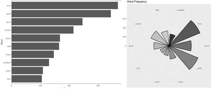
Frequents words in two different graphs
#frequent terms
frequent_terms <- freq_terms(data, top=10)
plot(frequent_terms)
write.table(frequent_terms,file="tabelashack.txt", sep=",")

#circular graph
Results<-dplyr::filter(frequent_terms, frequent_terms[,2]>20 )
colnames(Results)<-c("word", "frequency")
library(ggplot2)
ggplot2::ggplot(Results, aes(x=word, y=frequency, fill=word)) +
geom_bar(width = 0.75, stat = "identity", size = 1,color="black") +
 scale_fill_grey()+
coord_polar(theta = "x") + xlab("") + ylab("") + ggtitle("Word Frequency")
+ theme(legend.position = "none") + labs(x = NULL, y = NULL)

- By using the library(wordcloud) you can get a wordcloud with the most frequent words,wordcloud(word, n, max.words = 10, colors=pal2)
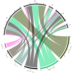
- chordDiagram provides a visual way of words frequency between companies
##graph circular
install.packages("circlize")
library(circlize)
read.csv("C:/......csv",sep=',')->a #contingency table, frequnecy of words by company
circos.clear()
circos.par(gap.after = c(rep(5, nrow(a[1:6,])-1), 15, rep(5, ncol(a[1:6,])-1), 15))
col_mat = rand_color(length(mat), transparency = 0.5)
chordDiagram(a[1:6,], directional = TRUE, transparency = 0, col = col_mat)
A really interesting example about how to perform tidy sentiment analysis in R on Prince’s songs. And other interesting pages:
- Basics of Text Mining in R – Bag of Words
- findMostFreqTerms: Find Most Frequent Terms
- Counting Words with R
- Text Mining with R
- Data Science 101: Sentiment Analysis in R Tutorial
- Text Analysis in R
- Text Mining: Sentiment Analysis
- Tidy Sentiment Analysis in R
- Spanish language: airbnb example
- An overview of keyword extraction techniques
